Set the publication parameters for this version
pub_range <- c(2001, 2023); program <- "TCRMP"; taxon_level <- "species"; version <- "aspublished"Territorial Coral Reef Monitoring Program, species level, 2001 to 2023
Olinger LK, Edmunds PJ, Levitan D, Smith TB, Lasker H, Feeley M, Mahoney L, Dahl A. Reproductive mode, but not rarity, influences population trajectories in corals. In Review 2026.
The coral-cover data for this analysis comes from the Reef Code benthic cover section: coral species cover download.
The Territorial Coral Reef Monitoring Program records coral cover at the species level across 20 shallow reef sites. Broadcast-spawning corals decline steeply, brooding corals decline slowly, and rare and common taxa decline at the same proportional rate. This page renders the published analysis over its paper range, 2001 through 2023. The full analysis runs below, from the coral-cover file to the figure (Figure 1) and the statistics table (Table 1). Every step is folded. Open any block to read the code and the plain-language notes.
pub_range <- c(2001, 2023); program <- "TCRMP"; taxon_level <- "species"; version <- "aspublished"suppressWarnings(suppressPackageStartupMessages({
library(tidyverse)
library(sandwich)
library(lmtest)
library(broom)
library(patchwork)
library(kableExtra)
}))
# The four analysis groups keep one color across every page. Warm hues mark
# brooders, cool hues mark broadcasters; the darker shade of each pair marks
# common taxa, the lighter marks rare.
palette_grp <- c(
"Common.Broadcaster" = "#0072B2", "Rare.Broadcaster" = "#56B4E9",
"Common.Brooder" = "#D55E00", "Rare.Brooder" = "#E69F00"
)
label_grp <- c(
"Common.Broadcaster" = "Common broadcaster", "Rare.Broadcaster" = "Rare broadcaster",
"Common.Brooder" = "Common brooder", "Rare.Brooder" = "Rare brooder"
)The analysis begins from the species-level coral-cover file and the site master table. The cover file holds one row per transect observation: a site, a year, a survey period, a coral species, and its percent cover. The site master holds each site’s program, depth, and the year monitoring began. The cover file is matched by pattern in data/cover/, so this step reads whichever species-level file is bundled, and the analysis grows as that file grows.
cover_files <- sort(list.files("../../data/cover", pattern = "s2pt5.*\\.csv$", full.names = TRUE))
cover_file <- tail(cover_files, 1)
benthiccover <- read.csv(cover_file) |>
  select(year, program, site, period, coralSpecies, perccover)
sitedat <- read.csv("../../data/site/00_RRS_siteMaster_allSites_data.csv")
c(cover_file = basename(cover_file), cover_rows = nrow(benthiccover), sites_listed = nrow(sitedat))
cover_file
"s2pt5_benthicCoverCoralSpecies_41sites_1999_2024.csv"
cover_rows
"481351"
sites_listed
"50" The first move is the explicit publication-range clip: every downstream step runs only on years inside pub_range. At the published range this clip is harmless, since the bundled file does not extend beyond it; as the cover file grows in later monitoring years, the same clip is what keeps this page reproducing the published analysis exactly. After the clip, the analysis holds the rest of the sampling design constant so that trends reflect coral change rather than changes in which reefs or taxa were surveyed: the shallow TCRMP sites established before 2006, the annual surveys, and the coral species identified to species. It drops the fire corals (Millepora), the generic catch-all entries, the Orbicella complex placeholder, and any taxon left at the genus level. The site scope comes first, because the cover scope depends on the surviving site list.
# Publication-range clip: the explicit first step of scope.
benthiccover <- benthiccover |> filter(year >= pub_range[1], year <= pub_range[2])

# Sites: shallow TCRMP reefs established before 2006 (Ginsburg Fringe excluded).
sitedat <- sitedat |>
  filter(program == "TCRMP", yearadded < 2006, site != "Ginsburg Fringe") |>
  mutate(depth_cat = ifelse(depth < 21, "Shallow", "Deep")) |>
  filter(depth_cat == "Shallow")

# Cover: TCRMP annual surveys.
benthiccover <- benthiccover |>
  filter(program == "TCRMP", period == "Annual")

# Taxa: fix one spelling, drop non-species and non-coral entries, keep scoped sites.
benthiccover <- benthiccover |>
  mutate(coralSpecies = ifelse(coralSpecies == "Orbicella franksii", "Orbicella franksi", coralSpecies)) |>
  filter(
    !coralSpecies %in% c("Millepora alcicornis", "Millepora complanata", "Millepora squarrosa",
                         "Coral spp.", "Juvenile coral spp.", "Orbicella species complex"),
    !grepl(" spp\\.$", coralSpecies),
    site %in% sitedat$site
  )
c(cover_rows = nrow(benthiccover), sites_kept = n_distinct(benthiccover$site),
  species = n_distinct(benthiccover$coralSpecies))
cover_rows sites_kept species
124411 20 49 Validation note: the scoped dataset spans 2001 through 2023, holds 124,411 transect records across 20 TCRMP sites and 49 coral species.
The analysis compares a baseline period to the full record. It bins the survey years into five-year groups and treats the first group as the baseline. Binning smooths the year-to-year noise in the baseline abundance ranking without changing the annual data used later in the model. The helper below builds the five-year groups from the data range and labels each year with its group.
# bin_years: label each year with a five-year group, dropping a trailing stub
# group so the last bin holds a full span where possible.
bin_years <- function(df, interval = 5) {
  min_yr <- min(df$year, na.rm = TRUE); max_yr <- max(df$year, na.rm = TRUE)
  breaks <- seq(min_yr, max_yr, by = interval)
  if (tail(breaks, 1) > max_yr - (interval - 1)) breaks <- head(breaks, -1)
  labels <- paste(breaks, pmin(breaks + (interval - 1), max_yr), sep = "-")
  map <- data.frame(year = seq(min_yr, max_yr)) |>
    mutate(year_group = cut(year, breaks = c(breaks, max_yr + 1), labels = labels,
                            right = FALSE, include.lowest = TRUE))
  df |> left_join(map, by = "year") |> mutate(year_group = as.factor(year_group))
}

benthiccover <- bin_years(benthiccover, 5)
earliest_year_group <- levels(benthiccover$year_group)[1]
# earliest_year_group
The baseline period is the first five-year group, 2001-2005. Two presence rules keep the analysis on taxa that were part of the community at baseline and at sites within their range. The first keeps species recorded during the baseline period. The second drops species-site pairs where the species was never seen, since a site outside a species range would enter the model as a structural zero rather than a decline.
# Every observed species x year-group (cover > 0), captured before the baseline filter so the
# excluded-taxa table (Step 15) can list taxa seen but absent from the baseline community.
species_yeargroup_observed <- benthiccover |>
  group_by(coralSpecies, year_group) |>
  summarize(seen = max(perccover, na.rm = TRUE) > 0, .groups = "drop") |>
  filter(seen)
# Keep species observed during the baseline period.
spp_in_baseline <- species_yeargroup_observed |>
  filter(year_group == earliest_year_group) |>
  pull(coralSpecies) |> unique()
benthiccover <- benthiccover |> filter(coralSpecies %in% spp_in_baseline)

# Drop species-site pairs where the species was never observed (out of range).
in_range <- benthiccover |>
  group_by(coralSpecies, site) |>
  summarize(seen = max(perccover, na.rm = TRUE) > 0, .groups = "drop") |>
  filter(seen) |> mutate(key = paste(coralSpecies, site))
benthiccover <- benthiccover |>
  filter(paste(coralSpecies, site) %in% in_range$key)

# Average across the transects at each site and year.
benthiccover <- benthiccover |>
  group_by(year_group, coralSpecies, year, site) |>
  summarise(perccover = mean(perccover, na.rm = TRUE), .groups = "drop")
c(rows = nrow(benthiccover), species = n_distinct(benthiccover$coralSpecies))
rows species
10073 40 Each species receives its mean percent cover during the baseline period. Ranking the species by that mean sets the order used in the figure and sets up the commonness split. The cumulative proportion of cover, summed down the ranked list, measures how much of the reef’s baseline cover the top species account for.
baseline <- benthiccover |>
  filter(year_group == earliest_year_group) |>
  group_by(coralSpecies) |>
  summarise(meancov = mean(perccover, na.rm = TRUE), .groups = "drop") |>
  arrange(desc(meancov)) |>
  mutate(rank = row_number(),
         normcov = meancov / sum(meancov, na.rm = TRUE),
         cumsumcov = cumsum(normcov))
# head(baseline, 6)The commonness split follows one rule: the species that together hold the top 90 percent of baseline cumulative cover are common, and the rest are rare. The manuscript identified 0.90 through a sliding-window analysis as the strictest rarity definition that leaves the temporal slopes stable.
baseline <- baseline |>
  mutate(commonness = ifelse(cumsumcov <= 0.900001, "Common", "Rare"))
table(baseline$commonness)
Common   Rare
10 30 Each species carries a reproductive mode, brooder or broadcaster. The assignment reads a compiled trait table, drops unknown entries, and joins the mode onto the baseline species. A second trait table fills any species the first leaves unassigned. Species that still lack a mode after both sources leave the analysis, because the model compares brooders to broadcasters and cannot place an unassigned species.
repro1 <- read.csv("../../data/collab/reproMode_coralSpecies_Mahoney_20250108.csv") |>
  rename(coralSpecies = Species) |>
  filter(Reproductive_mode %in% c("Brooder", "Broadcaster")) |>
  distinct(coralSpecies, Reproductive_mode)
repro2 <- read.csv("../../data/collab/reproMode_coralSpecies_Olinger_20250108.csv") |>
  filter(Reproductive_mode %in% c("Brooder", "Broadcaster")) |>
  distinct(coralSpecies, Reproductive_mode)

baseline <- baseline |>
  left_join(repro1, by = "coralSpecies") |>
  left_join(repro2, by = "coralSpecies", suffix = c("", ".2")) |>
  mutate(Reproductive_mode = coalesce(Reproductive_mode, Reproductive_mode.2)) |>
  select(-Reproductive_mode.2) |>
  filter(Reproductive_mode %in% c("Brooder", "Broadcaster"))
# with(baseline, table(Commonness = commonness, `Reproductive mode` = Reproductive_mode))The model works on group means rather than individual species, so that a single abundant species cannot dominate the trend. This step joins the commonness and reproductive-mode labels onto the full cover series, averages cover within each group at each site and year, adds a year index that starts at zero, and takes the log10 of cover. Log10 cover is the response, because coral loss acts proportionally, and a proportional change is a straight line on the log scale.
analysis_data <- benthiccover |>
  inner_join(baseline |> select(coralSpecies, commonness, Reproductive_mode), by = "coralSpecies") |>
  group_by(category = commonness, Reproductive_mode, year, site) |>
  summarise(perccover = mean(perccover, na.rm = TRUE), .groups = "drop") |>
  mutate(yearind = year - min(year), perccoverLog = log10(perccover)) |>
  filter(perccover > 0) |>
  mutate(category = factor(category, levels = c("Common", "Rare")),
         Reproductive_mode = factor(Reproductive_mode, levels = c("Broadcaster", "Brooder")))
c(model_rows = nrow(analysis_data), groups = nlevels(interaction(analysis_data$category, analysis_data$Reproductive_mode)))
model_rows groups
1442 4 The model predicts log10 percent cover from year, commonness, reproductive mode, and every interaction among them. Common and broadcaster are the reference levels, so the year term is the trend for common broadcasters, and the interactions measure how the other groups differ from it.
model_full <- lm(perccoverLog ~ yearind * category * Reproductive_mode, data = analysis_data)The residual variance is larger for the abundant groups than for the sparse groups, so ordinary standard errors would misstate the uncertainty. The analysis replaces them with HC3 heteroscedasticity-consistent standard errors, computed from a sandwich covariance matrix. Every standard error, p-value, and confidence interval below uses this robust covariance.
vcov_hc3 <- sandwich::vcovHC(model_full, type = "HC3")
coef_robust <- broom::tidy(lmtest::coeftest(model_full, vcov = vcov_hc3))The four group trends are linear combinations of the model coefficients. The common-broadcaster slope is the year term. Each other group adds the interactions that apply to it. The standard error of each slope comes from the robust covariance, so the uncertainty carries through. Annual percent change back-transforms the log10 slope into a yearly rate.
group_slope <- function(terms) {
  L <- setNames(rep(0, length(coef(model_full))), names(coef(model_full)))
  L[terms] <- 1
  est <- sum(L * coef(model_full))
  se <- sqrt(as.numeric(t(L) %*% vcov_hc3 %*% L))
  tibble(Slope = est, SE = se, `Annual % change` = 100 * (10^est - 1),
         `P-value` = 2 * pt(-abs(est / se), df = df.residual(model_full)))
}
group_slopes <- bind_rows(
  "Common broadcaster" = group_slope("yearind"),
  "Rare broadcaster"   = group_slope(c("yearind", "yearind:categoryRare")),
  "Common brooder"     = group_slope(c("yearind", "yearind:Reproductive_modeBrooder")),
  "Rare brooder"       = group_slope(c("yearind", "yearind:categoryRare",
                                       "yearind:Reproductive_modeBrooder",
                                       "yearind:categoryRare:Reproductive_modeBrooder")),
  .id = "Group"
)The figure pairs the baseline abundance distribution with the temporal trends. The left panel ranks species by baseline cover and colors each by group. The right panel shows site-level group mean cover over time on a log scale, with a linear fit per group.
sad_df <- baseline |>
  filter(meancov > 0) |>
  mutate(coralSpecies = factor(coralSpecies, levels = rev(baseline$coralSpecies[order(baseline$rank)])),
         grp = interaction(commonness, Reproductive_mode))
p_sad <- ggplot(sad_df, aes(coralSpecies, meancov, fill = grp)) +
  geom_col(width = 0.8) +
  scale_fill_manual(values = palette_grp, labels = label_grp, name = NULL, drop = FALSE) +
  coord_flip() +
  labs(x = NULL, y = "Mean baseline percent cover", title = "Baseline abundance") +
  theme_classic(base_size = 11) +
  theme(legend.position = "top", axis.text.y = element_text(face = "italic", size = 8))

trend_df <- analysis_data |> mutate(grp = interaction(category, Reproductive_mode))
p_trend <- ggplot(trend_df, aes(year, perccover, color = grp, fill = grp)) +
  geom_jitter(shape = 21, color = "black", alpha = 0.2, width = 0.25, height = 0, show.legend = FALSE) +
  geom_smooth(method = "lm", formula = y ~ x, se = TRUE, alpha = 0.15, linewidth = 0.8) +
  scale_color_manual(values = palette_grp, labels = label_grp, name = NULL, drop = FALSE) +
  scale_fill_manual(values = palette_grp, labels = label_grp, name = NULL, drop = FALSE) +
  scale_y_log10() + annotation_logticks(sides = "l", color = "grey70") +
  labs(x = "Year", y = "Percent cover (log scale)", title = "Temporal trends") +
  theme_classic(base_size = 11) +
  theme(legend.position = "top", axis.text.x = element_text(angle = 45, hjust = 1))

p_sad + p_trend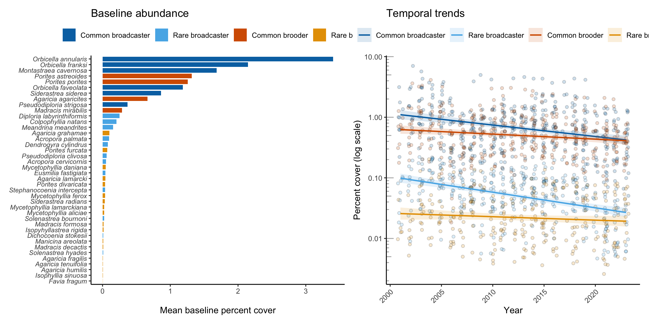
The table reports the model coefficients with HC3 robust standard errors and p-values. Bold marks terms significant at p less than 0.05.
term_labels <- c(
  "(Intercept)" = "Intercept", "yearind" = "Year",
  "categoryRare" = "Rarity", "Reproductive_modeBrooder" = "Repro. mode (brooder)",
  "yearind:categoryRare" = "Year x Rarity", "yearind:Reproductive_modeBrooder" = "Year x Repro. mode",
  "categoryRare:Reproductive_modeBrooder" = "Rarity x Repro. mode",
  "yearind:categoryRare:Reproductive_modeBrooder" = "Year x Rarity x Repro. mode"
)
coef_tbl <- coef_robust |>
  transmute(Predictor = term_labels[term],
            `Estimate (SE)` = sprintf("%.3f (%.3f)", estimate, std.error),
            `P-value` = ifelse(p.value < 0.001, "< 0.001", sprintf("%.3f", p.value)),
            .sig = p.value < 0.05)

kbl(coef_tbl |> select(-.sig), align = c("l", "r", "r"),
    caption = "Table 1 (TCRMP). Linear-model coefficients with HC3 robust standard errors.") |>
  kable_styling(bootstrap_options = c("striped", "hover", "condensed"), full_width = FALSE) |>
row_spec(which(coef_tbl$.sig), bold = TRUE)| Predictor | Estimate (SE) | P-value |
|---|---|---|
| Intercept | 0.042 (0.039) | 0.287 |
| Year | -0.019 (0.003) | < 0.001 |
| Rarity | -1.047 (0.056) | < 0.001 |
| Repro. mode (brooder) | -0.245 (0.055) | < 0.001 |
| Year x Rarity | -0.007 (0.005) | 0.141 |
| Year x Repro. mode | 0.011 (0.004) | 0.011 |
| Rarity x Repro. mode | -0.339 (0.084) | < 0.001 |
| Year x Rarity x Repro. mode | 0.009 (0.007) | 0.150 |
group_slopes |>
  mutate(Slope = sprintf("%.4f", Slope), SE = sprintf("%.4f", SE),
         `Annual % change` = sprintf("%.2f", `Annual % change`),
         `P-value` = ifelse(`P-value` < 0.001, "< 0.001", sprintf("%.3f", `P-value`))) |>
  kbl(align = c("l", "r", "r", "r", "r"),
      caption = "Group-specific temporal slopes estimated by Wald tests on linear combinations of model coefficients. The annual percent change is calculated as (10^slope - 1) x 100. P-values test the null hypothesis that the total temporal slope equals zero (H0: slope = 0). Common Broadcasters are the reference group; their slope and p-value come directly from the Year coefficient.") |>
kable_styling(bootstrap_options = c("striped", "hover", "condensed"), full_width = FALSE)| Group | Slope | SE | Annual % change | P-value |
|---|---|---|---|---|
| Common broadcaster | -0.0189 | 0.0032 | -4.26 | < 0.001 |
| Rare broadcaster | -0.0257 | 0.0033 | -5.75 | < 0.001 |
| Common brooder | -0.0083 | 0.0027 | -1.90 | 0.002 |
| Rare brooder | -0.0057 | 0.0038 | -1.31 | 0.131 |
The coefficient table reports the fitted trends. This table steps back to the species themselves and reports, for every taxon in the baseline community, how abundant and how widespread it was at the start of the record and how that changed by the end. Three complementary measures separate the different ways a species can decline. Cover is the mean percent cover across the species range. Occupancy is the proportion of surveyed sites where the species was present, so it tracks range contraction independent of local abundance. Local cover is the mean cover at the sites where the species was actually present, so it tracks thinning within the occupied range. A species can hold its occupancy while its local cover falls, or contract its range while staying dense where it persists; reporting both separates the two. Start values average over the baseline five-year group, and end values average over the last three years of the record. Occupancy counts a site only from the year it entered monitoring, so the denominator follows the site-by-site survey history rather than assuming every reef was watched from the first year.
source("../../_includes/_analysis_helpers.R")
species_table <- compute_change_metrics(benthiccover, baseline, sitedat, earliest_year_group, "coralSpecies")

.end_yrs <- (max(benthiccover$year) - 2):max(benthiccover$year)
.desc_tbl <- species_table |>
  arrange(rank_start) |>
  transmute(
    Species = taxon,
    `Repro. mode` = mode,
    Commonness = commonness,
    `Start rank` = rank_start,
    `End rank` = ifelse(is.na(rank_end), "-", as.character(rank_end)),
    `Start cover (%)` = sprintf("%.2f", cover_start),
    `End cover (%)` = ifelse(is.na(cover_end), "-", sprintf("%.2f", cover_end)),
    `Start occ. (%)` = sprintf("%.1f", occ_start),
    `End occ. (%)` = sprintf("%.1f", occ_end),
    `Start local cover (%)` = ifelse(is.na(ext_start), "-", sprintf("%.2f", ext_start)),
    `End local cover (%)` = ifelse(is.na(ext_end), "-", sprintf("%.2f", ext_end)),
    .common = commonness == "Common"
  )
kbl(.desc_tbl |> select(-.common), align = c("l", "l", "l", rep("r", 8)),
    caption = sprintf(
      "Descriptive statistics for coral species in the TCRMP monitoring program. Species are ordered by their rank in the baseline period (%s). Reproductive Mode ('Repro. Mode') indicates reproductive strategy. Rows in bold signify common species, determined by the top 90%% cumulative cover threshold during the baseline period. Start Cover (%%), Start Occupancy (Start Occup. (%%)), Start Local cover (%%), and Start Rank are metrics from the baseline period. End Cover (%%), End Occupancy (End Occup. (%%)), End Local cover (%%), and End Rank are metrics for the recent period (%d-%d).",
      earliest_year_group, min(.end_yrs), max(.end_yrs))) |>
  kable_styling(bootstrap_options = c("striped", "hover", "condensed"), full_width = FALSE) |>
  column_spec(1, italic = TRUE) |>
row_spec(which(.desc_tbl$.common), bold = TRUE)| Species | Repro. mode | Commonness | Start rank | End rank | Start cover (%) | End cover (%) | Start occ. (%) | End occ. (%) | Start local cover (%) | End local cover (%) | |
|---|---|---|---|---|---|---|---|---|---|---|---|
| Orbicella annularis | Orbicella annularis | Broadcaster | Common | 1 | 1 | 3.40 | 1.27 | 67.2 | 80.0 | 5.00 | 1.59 |
| Orbicella franksi | Orbicella franksi | Broadcaster | Common | 2 | 6 | 2.15 | 0.35 | 65.8 | 70.0 | 2.95 | 0.50 |
| Montastraea cavernosa | Montastraea cavernosa | Broadcaster | Common | 3 | 8 | 1.69 | 0.16 | 88.9 | 63.3 | 1.76 | 0.26 |
| Porites astreoides | Porites astreoides | Brooder | Common | 4 | 2 | 1.32 | 1.19 | 90.4 | 98.3 | 1.36 | 1.21 |
| Porites porites | Porites porites | Brooder | Common | 5 | 5 | 1.26 | 0.36 | 81.4 | 86.7 | 1.44 | 0.41 |
| Orbicella faveolata | Orbicella faveolata | Broadcaster | Common | 6 | 3 | 1.18 | 0.62 | 58.0 | 75.0 | 1.86 | 0.83 |
| Siderastrea siderea | Siderastrea siderea | Broadcaster | Common | 7 | 4 | 0.86 | 0.37 | 88.1 | 80.0 | 0.92 | 0.46 |
| Agaricia agaricites | Agaricia agaricites | Brooder | Common | 8 | 7 | 0.66 | 0.27 | 80.4 | 75.0 | 0.75 | 0.36 |
| Pseudodiploria strigosa | Pseudodiploria strigosa | Broadcaster | Common | 9 | 11 | 0.37 | 0.05 | 63.9 | 31.7 | 0.52 | 0.16 |
| Madracis mirabilis | Madracis mirabilis | Brooder | Common | 10 | 17 | 0.29 | 0.01 | 19.4 | 11.7 | 1.03 | 0.12 |
| Diploria labyrinthiformis | Diploria labyrinthiformis | Broadcaster | Rare | 11 | 16 | 0.25 | 0.01 | 51.6 | 11.7 | 0.43 | 0.12 |
| Colpophyllia natans | Colpophyllia natans | Broadcaster | Rare | 12 | 18 | 0.21 | 0.01 | 47.2 | 15.0 | 0.44 | 0.06 |
| Meandrina meandrites | Meandrina meandrites | Broadcaster | Rare | 13 | - | 0.15 | 0.00 | 46.1 | 0.0 | 0.29 | - |
| Agaricia grahamae | Agaricia grahamae | Brooder | Rare | 14 | 26 | 0.10 | 0.00 | 4.2 | 1.7 | 0.72 | 0.04 |
| Acropora palmata | Acropora palmata | Broadcaster | Rare | 15 | 29 | 0.10 | 0.00 | 2.9 | 1.7 | 0.39 | 0.02 |
| Dendrogyra cylindrus | Dendrogyra cylindrus | Broadcaster | Rare | 16 | - | 0.08 | 0.00 | 15.9 | 0.0 | 0.25 | - |
| Porites furcata | Porites furcata | Brooder | Rare | 17 | 14 | 0.07 | 0.02 | 14.0 | 21.7 | 0.31 | 0.10 |
| Pseudodiploria clivosa | Pseudodiploria clivosa | Broadcaster | Rare | 18 | 27 | 0.06 | 0.00 | 22.1 | 1.7 | 0.23 | 0.04 |
| Acropora cervicornis | Acropora cervicornis | Broadcaster | Rare | 19 | 21 | 0.05 | 0.00 | 4.0 | 6.7 | 0.39 | 0.05 |
| Mycetophyllia daniana | Mycetophyllia daniana | Brooder | Rare | 20 | - | 0.05 | 0.00 | 10.7 | 0.0 | 0.12 | - |
| Eusmilia fastigiata | Eusmilia fastigiata | Broadcaster | Rare | 21 | 24 | 0.04 | 0.00 | 21.9 | 3.3 | 0.13 | 0.02 |
| Agaricia lamarcki | Agaricia lamarcki | Brooder | Rare | 22 | 9 | 0.04 | 0.08 | 11.5 | 35.0 | 0.23 | 0.23 |
| Porites divaricata | Porites divaricata | Brooder | Rare | 23 | 13 | 0.04 | 0.03 | 16.5 | 21.7 | 0.17 | 0.13 |
| Stephanocoenia intercepta | Stephanocoenia intercepta | Broadcaster | Rare | 24 | 10 | 0.04 | 0.07 | 17.7 | 50.0 | 0.17 | 0.14 |
| Mycetophyllia ferox | Mycetophyllia ferox | Brooder | Rare | 25 | - | 0.04 | 0.00 | 6.5 | 0.0 | 0.18 | - |
| Siderastrea radians | Siderastrea radians | Brooder | Rare | 26 | 22 | 0.03 | 0.00 | 19.2 | 3.3 | 0.15 | 0.06 |
| Mycetophyllia lamarckiana | Mycetophyllia lamarckiana | Brooder | Rare | 27 | - | 0.03 | 0.00 | 4.4 | 0.0 | 0.14 | - |
| Mycetophyllia aliciae | Mycetophyllia aliciae | Brooder | Rare | 28 | 20 | 0.02 | 0.00 | 5.0 | 5.0 | 0.13 | 0.08 |
| Solenastrea bournoni | Solenastrea bournoni | Broadcaster | Rare | 29 | 23 | 0.02 | 0.00 | 8.6 | 3.3 | 0.13 | 0.04 |
| Madracis formosa | Madracis formosa | Brooder | Rare | 30 | - | 0.01 | 0.00 | 1.5 | 0.0 | 0.11 | - |
| Isopyhyllastrea rigida | Isopyhyllastrea rigida | Brooder | Rare | 31 | - | 0.01 | 0.00 | 1.5 | 0.0 | 0.07 | - |
| Dichocoenia stokesii | Dichocoenia stokesii | Broadcaster | Rare | 32 | - | 0.01 | 0.00 | 6.7 | 0.0 | 0.11 | - |
| Manicina areolata | Manicina areolata | Brooder | Rare | 33 | 28 | 0.01 | 0.00 | 3.7 | 1.7 | 0.07 | 0.04 |
| Madracis decactis | Madracis decactis | Brooder | Rare | 34 | 12 | 0.01 | 0.03 | 9.8 | 38.3 | 0.11 | 0.08 |
| Solenastrea hyades | Solenastrea hyades | Broadcaster | Rare | 35 | - | 0.01 | 0.00 | 1.5 | 0.0 | 0.15 | - |
| Agaricia fragilis | Agaricia fragilis | Brooder | Rare | 36 | 25 | 0.01 | 0.00 | 1.5 | 1.7 | 0.16 | 0.05 |
| Agaricia tenuifolia | Agaricia tenuifolia | Brooder | Rare | 37 | 19 | 0.01 | 0.01 | 2.3 | 1.7 | 0.13 | 0.53 |
| Agaricia humilis | Agaricia humilis | Brooder | Rare | 38 | 15 | 0.01 | 0.02 | 1.5 | 15.0 | 0.32 | 0.10 |
| Isophyllia sinuosa | Isophyllia sinuosa | Brooder | Rare | 39 | - | 0.00 | 0.00 | 0.0 | 0.0 | 0.07 | - |
| Favia fragum | Favia fragum | Brooder | Rare | 40 | - | 0.00 | 0.00 | 1.2 | 0.0 | 0.05 | - |
The analysis objects are written to a timestamped RData file under data/rdata/, tagged with the program and the version (as published or updated) so the two ranges never overwrite each other. The manuscript-values page loads the most recent file for each program and version and reads every derived number from these saved objects, rather than repeating the computation. The derived CSVs written elsewhere are left unchanged.
The trend model runs only on species that were part of the baseline community, so that a modeled slope reflects a species present at the outset rather than one that arrived mid-record. Some species were observed at least once during the record but not during the baseline period, or could not be assigned a reproductive mode; those are held out of the trend analysis and listed here with the year each was first observed.
.excl <- excluded_taxa_table(species_yeargroup_observed, baseline$coralSpecies, "coralSpecies")
kbl(.excl, align = c("l", "r"),
    caption = "Taxa excluded from trend analyses because they were not recorded during the baseline period (2001–2005 for TCRMP and VINPS; 1992–1996 for CSUN). For each taxon, the program and year of first observation at shallow monitoring sites are shown. CSUN taxa are at the genus level; TCRMP and VINPS taxa are at the species level.") |>
  kable_styling(bootstrap_options = c("striped", "hover", "condensed"), full_width = FALSE) |>
column_spec(1, italic = TRUE)| Taxon | Year first observed |
|---|---|
| Helioseris cucullata | 2006 |
| Oculina diffusa | 2016 |
| Scolymia cubensis | 2006 |
| Scolymia lacera | 2011 |
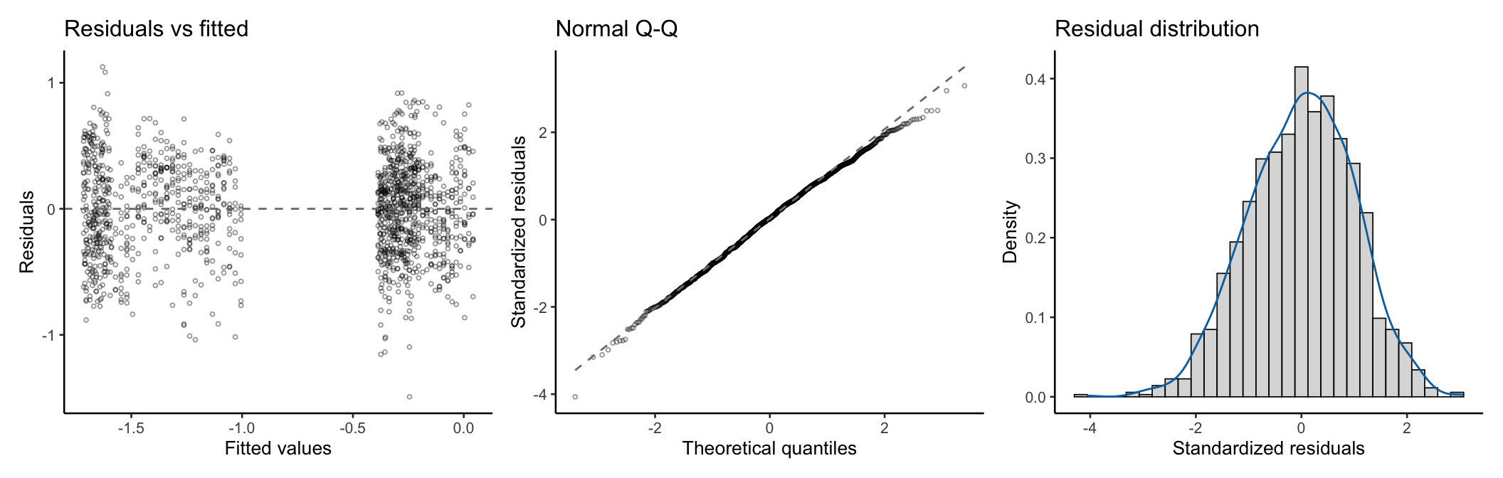
The coefficient table uses HC3 robust standard errors because the residual variance is not constant across groups. These diagnostic panels show why. Residuals versus fitted values reveal the unequal spread, the normal Q-Q plot shows the tails, and the residual distribution summarizes the whole. The robust standard errors used throughout the analysis are the response to exactly this structure.
model_diagnostics_plot(model_full)